a primer on embedded manifolds

The possibility of applying geometric techniques to machine learning is what originally sparked my interest in the latter subject. Using such methods, the goal is to inject spatial intuition into mathematical machine learning, which is often presented—at least in many introductory textbooks—as an almost purely analytical subject, with a heavy reliance on probability theory. A prime and very simple example of geometric intuition applied to machine learning is the familiar description of the gradient descent algorithm as walking downhill to find the minimum. In this description, you are being asked to visualize the graph of the objective function, and therefore to conceive of the function as a geometric object, and not purely an analytic one. The geometry lends insight and explains why the algorithm works.

The possibilities of using geometry in machine learning go well beyond the basic gradient descent algorithm, however, and finding new and interesting geometric applications in machine learning is an active and exciting area of contemporary research. For example, there are several papers appearing in recent proceedings of the ICML (from the “Topology, Algebra, and Geometry in Machine Learning” workshop) that I want to explore in future posts in this blog. In addition, there is the fascinating area of so-called geometric deep learning (see here and here), that I’d like to begin exploring.

I am using the word geometry in a very broad sense—in particular, I am not referring to Euclid’s plane geometry that you studied in high school, so you can put away your protractor and compass. Rather, I am using the word essentially as a synonym for topology, which is a branch of mathematics that might be described as abstract geometry. Topology provides us the abstract framework to talk about “geometric” properties like smoothness and dimensionality in very general settings, and it gives us the tools to assemble “spaces” out of quite general things, like probability distributions. In fact, “spaces” of probability distributions are the central objects in information geometry, where they go by the name statistical manifolds.

The cutting-edge applications of geometry and topology to machine learning will have to come later, however. We have a good amount of preparatory work that we need to do before we can get to the research boundary. In this entirely mathematical¹ series of posts, I want to give you a glimpse into the various branches of topology and modern geometry, helping develop familiarity with some of the basic objects that appear in geometric and topological machine and deep learning.

In this first post, we will begin by discussing embedded smooth manifolds, which make for a good introduction to topology due to their concreteness. We will stick with embedded manifolds for a few posts, using the ambient cartesian spaces as a concrete setting in which to learn the rudiments of the theory. Later, we will remove our reliance on the ambient cartesian spaces and consider instead general abstract manifolds. The theory of these more general manifolds can be much more difficult, but having learned about embedded manifolds beforehand, we will have no problems!

Table of contents

1. Basic definitions
2. Tangent spaces and derivatives/pushforwards
3. Further reading
4. References and footnotes

Prerequisites

Though I want to minimize the prerequisites for this series of posts as much as possible, I have to begin somewhere. If I were to assume no training in mathematics beyond, say, basic single-variable calculus, then I would have to write an entire book to ultimately get where I want to go.

Therefore, I’ve pitched these posts at the level of a junior or senior mathematics major. I’m assuming that you’ve had a full sequence of calculus (including multi-variable calculus), as well as a good course in linear algebra and abstract vector spaces and linear transformations. It will also be very helpful to be familiar with the basic definitions and results in the first chapter of Guillemin and Pollack’s Differential Topology.²

You will also need to know the definition of commutative $\bbr$-algebras and their homomorphisms. You can look up these definitions on the internet, or see the section on Further Reading.

The entire theory that we will develop is based on the notion of smoothness. Therefore, the following definition is absolutely fundamental:

For example, the function

is smooth, precisely because the two component functions

are polynomials, which are smooth. Can you write down other examples of smooth functions?

Notice that I am writing superscripts to index the component functions, rather than (the more typical) subscripts. In particular, $\alpha^2$ does not stand for “$\alpha$ squared”, but rather for the second component function of $\alpha$. As we will see later, the placement of indices in superscripts versus subscripts will be significant.

While reading the definition, you may have wondered if the two definitions of smoothness coincide when $M$ is open. In other words, you may have asked: If $\alpha:M \to N$ is a function on an open set $M$ which is smooth according to part (1.) of the definition, is it also smooth according to part (2.)? I suggest that you prove the answer is yes, and to also prove the converse, so that the two definitions are equivalent when $M$ is open.

We will need special types of smooth functions in order to define smooth manifolds:

If two sets $M$ and $N$ are linked by a diffeomorphism $\alpha:M \to N$ (so that they are diffeomorphic), then, from our viewpoint, they are to be considered indistinguishable or “the same.” In other words, the type of topology that we are studying only considers properties of sets $M$ and $N$ that are invariant under diffeomorphism, in the sense that if $M$ has such and such property, then so does $N$ (provided $M$ and $N$ are diffeomorphic).

As an (extremely simple) example, the real line $\bbr$ and the parabola

are diffeomorphic via the map $\alpha: \bbr \to N$ with $x\mapsto (x, x^2)$. Can you prove that $\alpha$ is smooth, and identify its (smooth) inverse?

Armed with the definition of a diffeomorphism, we arrive at the main definition:

The cartoon to keep in mind is the following:

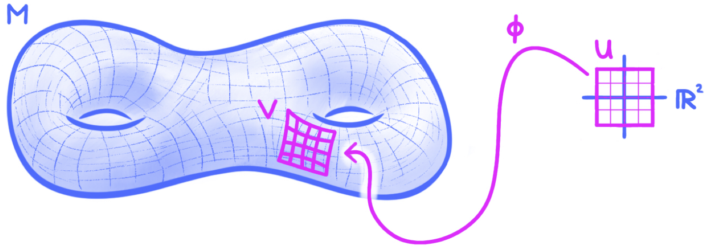
Here, I’ve drawn $M$ as a $2$-dimensional smooth manifold (in particular, a “two-holed torus”). You should imagine that the diffeomorphism $\phi$ is “painting” a set of local coordinate axes on $M$. Though this figure only shows one such diffeomorphism, the definition requires that the entire manifold $M$ is covered with these local coordinate systems. In other words, no matter what point $p\in M$ I choose, there is a diffeomorphism $\phi: U \to V$ as in the figure with $p \in V$.

Our smooth manifolds carry the subspace topologies from their ambient cartesian spaces, so the open neighborhood $V$ in the definition is a relatively open subset of $M$. A diffeomorphism $\phi$ as in the definition is called a local parameterization on $M$ and its inverse $\phi^{-1}:V\to U$ is called a local coordinate system or a chart on $M$. The coordinate functions $(\phi^{-1})^i:V\to \bbr$ ($i=1,\ldots,n$) are often suggestively written as

which are often (intentionally) confused with the map $\phi^{-1}$ itself and called local coordinates or a local coordinate system on $M$. Given a point $p\in M$, we shall say that \eqref{local-coord-eqn} are local coordinates near $p$ if $p$ is in the domain $V$ of the local coordinate system $\phi^{-1}$.

Often we shall omit the modifier “smooth” and simply write “manifold” when we really mean “smooth manifold.”

As with any category of mathematical objects, it’s not enough to only define the objects, but we also need to define the appropriate maps between them:

So, a typical smooth map between manifolds might look something like this:

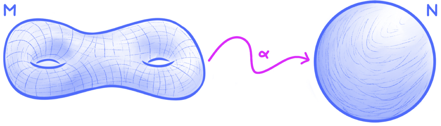
Here, $\alpha:M \to N$ is a smooth map that sends a “two-holed” torus $M$ to a sphere $N$ (i.e., the surface of a ball). I tend to picture smooth maps as dynamic processes that somehow bend, twist or otherwise transform the domain manifold to land in (or on) the codomain manifold. So, I would picture $\alpha$ as some sort of (smooth) transformation that places the two-holed torus $M$ onto the surface of the sphere $N$. As an extreme example, $\alpha$ could collapse all of $M$ to a point, and then map that point to the north pole of $M$. Can you picture other examples for what $\alpha$ might do?

Though not always rigidly observed and followed, in some branches of topology and geometry it is traditional to use the word “function” as a stand-in for “$\bbr$-valued”, so that a smooth function on a manifold $M$ is a smooth map $\alpha:M \to \bbr$. The set of such smooth functions is so important that it has its own special notation:

In fact, given a manifold $M$, the set $C^\infty(M)$ of smooth functions is a commutative $\bbr$-algebra with respect to the standard pointwise operations: Given two functions $f,g\in C^\infty(M)$, their sum, denoted $f+g$, is defined via the formula

for all $p\in M$, while their product, denoted $fg$, is defined via the formula

for all $p\in M$. Then, given a scalar $c\in \bbr$, we define the scalar product of $c$ and $f$, denoted $cf$, via the formula

for all $p\in M$.

In the next exercise, I want you to check that $C^\infty(M)$ actually is a commutative $\bbr$-algebra and several other things.

A cartoon illustrating the mechanics of a pullback of a smooth map is shown here:

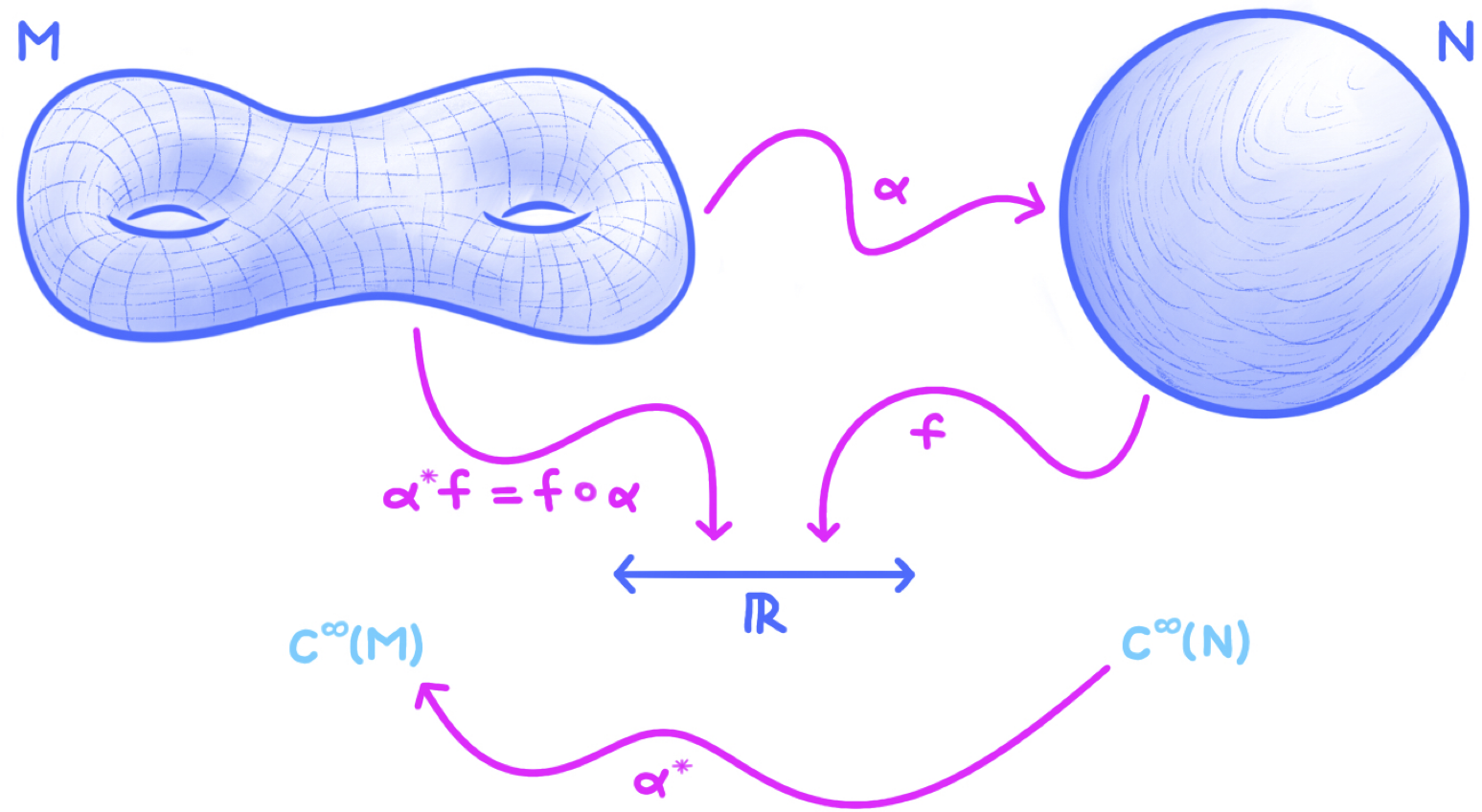
The smooth function $f: N\to \bbr$ is defined on the codomain manifold of the smooth map $\alpha$. Notice that $f$ maps to the real line $\bbr$ in the figure, and so does $\alpha^\ast f:M \to \bbr$. The smooth map $\alpha$ maps from $M$ to $N$, but the pullback $\alpha^\ast$ goes backwards, mapping $C^\infty(N)$ to $C^\infty(M)$. This “reversal of directions” is an example of (functorial) contravariance.

The last part of the exercise is significant because it shows that the algebras of smooth functions of manifolds are diffeomorphism invariants. Thus, if you want to show that two manifolds are not diffeomorphic, you can do so by showing that their algebras of smooth functions are not isomorphic. The latter may not be any easier than the former, but it’s still quite interesting because it shows that the pullback operation turns a topological problem (the non-existence of a diffeomorphism) into an algebraic problem (the non-existence of an isomorphism).³

If the pullback operation turns a smooth map into an algebra homomorphism pointing in the “opposite direction,” then the pushforward operation turns a smooth map into a homomorphism of vector spaces pointing the “same direction.” In particular, pushforwards also turn topology into (linear) algebra.

Pushforwards aren’t really that mysterious, since they are nothing but directional derivatives with a fancy name, and you certainly know what a derivative is. So, let’s begin by recalling the definition of derivatives on open sets in cartesian space:

With $\phi$ given as in the definition, and with respect to the standard ordered bases on $\bbr^s$ and $\bbr^r$, one may prove easily that the derivative $\phi_{\ast t}$ is represented by the $r\times s$ jacobian matrix

where $t^1,\ldots,t^s$ are the standard ordered coordinates⁴ on $\bbr^s$. For more details, see Chapter 2 of (⁵).

The tangent spaces to a manifold are the direct generalizations of the tangent lines and planes that you studied in single- and multi-variable calculus.

The rather strange choice of notation for the coordinate basis vectors will be explained when we study the relationship between tangent vectors and derivations in a later post. However, notice that the index $i$ appears in the subscript of the coordinate basis vector $\bd_{x^i}|_p$, which means that we consider it to be a lower index on this basis vector. One often sees the convention that stipulates that an index repeated in a single expression in both an upper and lower position is to be summed over. In view of this convention, a tangent vector $v\in T_p(M)$ may be written in components as

with summation over $i$ implied (from $1$ to $n$). When specific mention of the local coordinates is not necessary, we will write $\bd_i|_p$ in place of $\bd_{x^i}|_p$.

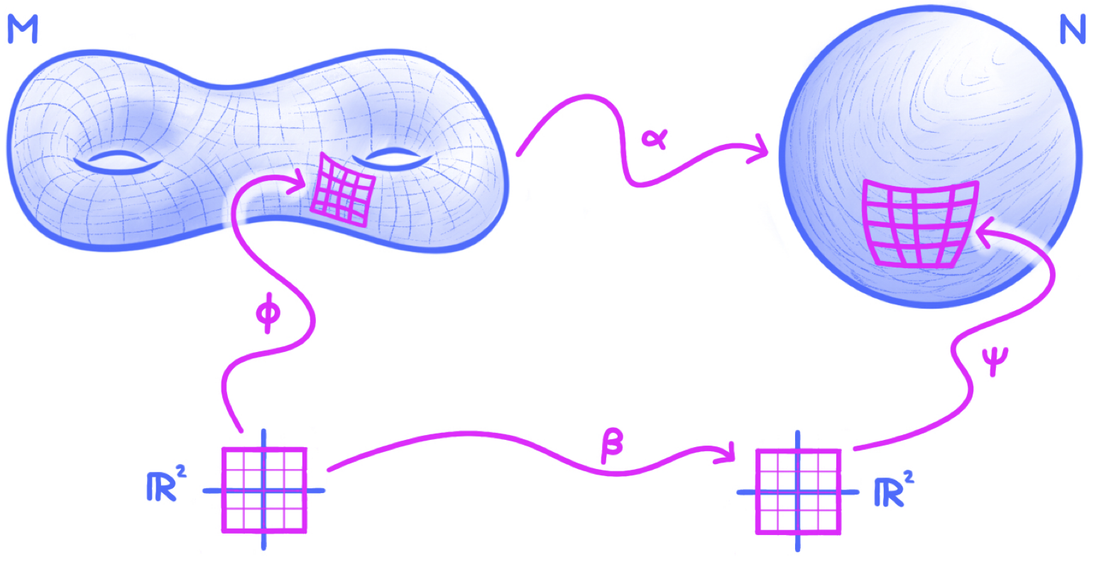
Now, having defined pushforwards of smooth maps defined on open subsets of cartesian spaces, we generalize to pushforwards of smooth maps between manifolds. So, let $\alpha:M \to N$ be a smooth map between manifolds, let $p\in M$, and set $q = \alpha(p)$. We may choose local parametrizations

on $M$ and $N$, respectively, with $p\in V$ and $q\in G$. By shrinking $U$ and $V$ if needed, we may suppose that $\alpha(V) \subseteq G$. Thus, the diagram

is well-defined and commutes. If $x^1,\ldots,x^n$ and $y^1,\ldots,y^m$ are the local coordinates on $M$ and $N$ associated with the parametrizations $\phi$ and $\psi$ (hence $M$ is $n$-dimensional while $N$ is $m$-dimensional), then the composite $\beta$ along the bottom of the diagram is called the local coordinate representation of $\alpha$ with respect to the $x^j$’s and $y^i$’s; a cartoon representation of the situation is given in the figure:

The jacobian matrix of $\beta$ at the point $\phi^{-1}(p)$ is denoted

The cartoon representation of the derivative is:

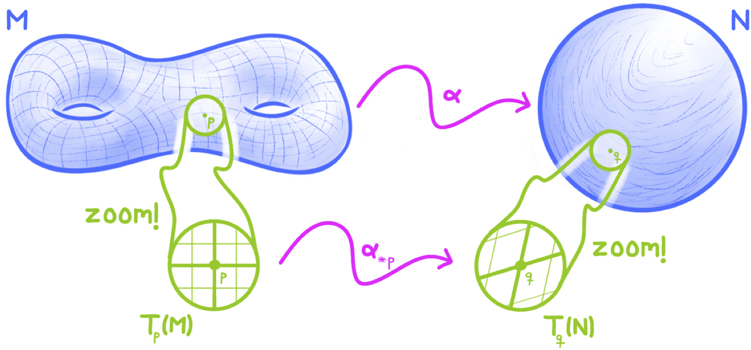
To the extent that the tangent spaces $T_p(M)$ and $T_q(N)$ can be considered “infinitesimal” neighborhoods of $p$ and $q$, the action of the smooth map $\alpha$ on these neighborhoods is given by a linear transformation $\alpha_{\ast p} : T_p(M) \to T_q(N)$.

The following fundamental result is proved on page 11 of (²):

As a sanity check, can you recover the usual single-variable chain rule from this version as a special case? I suggest you try!

Now, the derivative of a smooth map between open sets of cartesian spaces may be represented by a jacobian matrix. The same is true for smooth maps between manifolds, but in general, this matrix will depend on the choice of local coordinates. In fact, these jacobian matrices actually coincide with the jacobian matrices of the local coordinate representations as defined above. The first step to obtaining these jacobian matrices is to define partial derivatives of functions on a manifold, which also depend on the choice of local coordinates.

In the next exercise, you will work out, for yourself, the relationship between partial derivatives of component functions of smooth maps and jacobian matrices.

In my opinion, the best introduction to topology is Guillemin and Pollack’s book Differential Topology.² My treatment of (embedded) smooth manifolds in the first few posts of this series will closely follow the first chapter of this book. A pair of very good related texts is Spivak’s Calculus on Manifolds⁵ and Milnor’s Topology from the Differential Viewpoint.⁹

For the material in this post on commutative $\bbr$-algebras, see MacLane and Birkhoff’s Algebra¹⁰, particularly Chapter IX.