tangent bundles

The tangent space $T_p(M)$ at a point $p$ on a manifold $M$ is a purely local object, in the sense that it only depends on the “first-order infinitesimal neighborhoods” of $p$. In this post, we will see how to combine all the tangent spaces $T_p(M)$ into a single global object called the tangent bundle, denoted $T(M)$. While the tangent bundle $T(M)$ is composed of linear building blocks (i.e., the tangent spaces $T_p(M)$), we will see that $T(M)$ carries its own manifold structure which may have a non-trivial topology. As an example, we will explore the tangent bundle $T(S^1)$ of the unit circle $S^1$ in some detail, and we will see that $T(S^1)$ is a cylinder in $\bbr^3$.

A tangent bundle is actually a specific example of a more general structure called a (locally trivial) vector bundle, which are ubiquitous in topology. I will only have the time to state the definitions and most basic properties of these gadgets; a more thorough exploration will have to wait till a future post.

Table of contents

1. The tangent bundle
2. The tangent bundle of the circle
3. Tangent bundles as vector bundles
4. Tangent bundles as locally trivial vector bundles
5. References and footnotes

Prerequisites

Of course, you’ll want to be familiar with the basic definitions, notation, and terminology in the first post of this series. In particular, our manifolds are embedded in cartesian spaces by definition, in the style of Guillemin and Pollack’s book (¹), which will make for a handy reference for this post.

As a set, the tangent bundle is very easy to define. However, the tangent bundle carries an entire smooth manifold structure, which takes some time and care to define properly. While you’re working through this section, I recommend taking a peek at the section following this one (and its figure), which gives a concrete example of a tangent bundle.

As I mentioned, the tangent bundle $T(M)$ is more than just a subset of $\bbr^{2r}$, it’s actually a $2n$-dimensional smooth manifold. To see this, we first note that the assignment $M \mapsto T(M)$ is functorial: If $\alpha:M \to N$ is a smooth map, then there is an induced map

\begin{equation}\notag \alpha_\ast:T(M) \to T(N), \quad (p,v) \mapsto \big(\alpha(p),\alpha_{\ast p}(v)\big), \end{equation}

that we call the global derivative or global pushforward of $\alpha$. One checks easily that $\alpha_\ast$ is smooth, i.e., that it is locally extendible at each point $(p,v) \in T(M)$ to a smooth map on an open neighborhood of $(p,v)$ in $\bbr^{2r}$. Furthermore, by the usual chain rule, if $\beta:N \to L$ is a second smooth map, we have

\begin{equation}\notag (\beta\circ \alpha)_\ast = \beta_\ast \circ \alpha_\ast, \end{equation}

and if $\id_M:M \to M$ is the identity map, then

\begin{equation}\notag \id_{M\ast} = \id_{T(M)}. \end{equation}

It follows immediately, as usual, that if $\alpha:M \to N$ is a diffeomorphism, then $\alpha_\ast$ is too.

Now, to get local parametrizations on $T(M)$, we let $\phi:U\to V$ be a local parametrization on $M$, where $U$ is an open subset of $\bbr^n$ and $V$ is an open subset of $M$. We then have the global derivative

\begin{equation}\notag \phi_\ast: T(U) \to T(V) \end{equation}

which we just saw is a diffeomorphism. Because we may identify each tangent space $T_t(U)$ with $\bbr^n$ ($t\in U$), we have that $T(U) = U \times \bbr^n$, and hence $T(U)$ is an open subset of $\bbr^{2n}$. On the other hand, because $V$ is open in $M$ and $T_p(V) = T_p(M)$ for all $p\in V$, we have

\begin{equation}\notag T(V) = (V \times \bbr^N) \cap T(M), \end{equation}

so $T(V)$ is an open subset of $T(M)$. We may thus take the global derivatives $\phi_\ast$ of local parametrizations of $M$ to obtain local parametrizations of $T(M)$, giving the latter the structure of a $2n$-dimensional manifold.

From this description, we can easily describe local coordinates on the codomain of a local parametrization $\phi_\ast:T(U) \to T(V)$. First, recall (from the first post) that the associated local coordinates $x^1,\ldots,x^n$ on the open subset $V\subseteq M$ are, by definition, the component functions of the inverse function $\phi^{-1}$, namely

\begin{equation}\notag \phi^{-1}(p) = (x^1(p),\ldots,x^n(p)), \end{equation}

for all $p\in V$. It is quite common to intentionally confuse the numbers $x^1(p),\ldots,x^n(p)$ with the functions $x^1,\ldots,x^n$ themselves, so that we might say (for example) the point $p\in V$ (on a $3$-dimensional manifold) has local coordinates

\begin{equation}\notag (x^1,x^2,x^3) = (-2, 3, 0), \end{equation}

when what we really mean is that

\begin{equation}\notag (x^1(p),x^2(p),x^3(p)) = (-2, 3, 0). \end{equation}

With respect to the local parametrization $\phi$, we also talked about the associated coordinate basis

\begin{equation} \label{tan-basis-eqn} \bd_1|_p,\ldots,\bd_n|_p \end{equation}

of the tangent space $T_p(M)$ at a point $p\in V$. Thus, every vector $v\in T_p(V)$ may be written as

\begin{equation} \label{tan-comp-eqn} v = v^i \bd_i|_p \end{equation}

for some (unique) collection of scalars $v^i \in \bbr$, with summation over $i$ implied.

Now, it follows immediately from our discussion that a point $(p,v) \in T(V) \subseteq T(M)$ has local coordinates given by

\begin{equation} \label{hor-ver-eqn} (x^1,\ldots,x^n,v^1,\ldots,v^n) \in \bbr^{2n}. \end{equation}

Take care to make sure you understand what this means! First, I am intentionally confusing the functions $x^1,\ldots,x^n$ with the numbers $x^1(p),\ldots,x^n(p)$ as I mentioned above, and the numbers $v^1,\ldots,v^n$ are the components of $v$ displayed in \eqref{tan-comp-eqn} with respect to the associated coordinate basis \eqref{tan-basis-eqn}.

Local coordinates of the form \eqref{hor-ver-eqn} are so important that they get their own name:

The language in the definition is the first of many “vertical/horizontal” dichotomies that you’d see if you continued your study of vector and fiber bundles. This language comes from how we typically draw tangent bundles, as we will see in the next section.

Given a point $p = (x,y) \in S^1$, where $S^1$ denotes the unit circle in $\bbr^2$, it’s easy to see that

\begin{equation}\notag T_p(S^1) = \left\{ (u,v) \in \bbr^2 \mid xu+yv = 0 \right\}. \end{equation}

Thus

\begin{equation}\notag T(S^1) = \left\{ (x,y,u,v) \in \bbr^4 \mid x^2+y^2 = 1, \ xu + yv = 0 \right\}. \end{equation}

Now, this is all well and good, but I actually want to find a different description of $T(S^1)$. For this, we define a smooth map

\begin{equation}\notag \alpha: S^1 \times \bbr \to T(S^1) \end{equation}

by setting

\begin{equation}\notag \alpha(x,y,r) = ( x,y , -yr,xr ). \end{equation}

One shows easily that $\alpha$ is an injective immersion, and that it is also proper; hence, $\alpha$ is an embedding. But its image is easily seen to be all of $T(S^1)$, which means that it is a diffeomorphism. Thus, at least up to diffeomorphism, the tangent bundle $T(S^1)$ is the same thing as the infinite cylinder $S^1 \times \bbr$.

The structure of the tangent bundle is shown in the following figure:

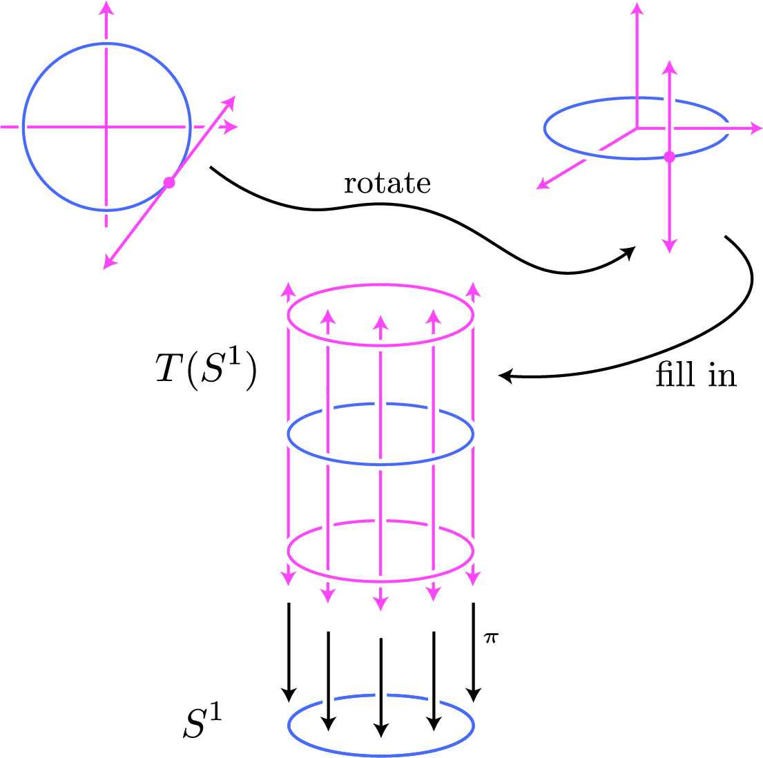
In the upper left, we begin with a single tangent line to the circle $S^1$ at a point in the fourth quadrant. Moving to the upper right, we view the circle $S^1$ as embedded in the $xy$-plane in $\bbr^3$, and we physically grab the tangent line and rotate it so that it is parallel with the $z$-axis. Then, if we imagine rotating all tangent lines to $S^1$ in this manner, we “fill in” the infinite cylinder $S^1 \times \bbr$, which is shown in the center of the figure labeled as $T(S^1)$.

At the bottom of the figure, I have drawn a copy of $S^1$ and placed it below the tangent bundle $T(S^1)$. This is a very typical convention, where we imagine (and sometimes actually draw, if possible) the tangent bundle $T(M)$ sitting “over” the manifold $M$. In fact, the manifold $M$ is sometimes called the base manifold of the bundle $T(M)$, because of this vertical orientation.

I have also drawn the smooth map

\begin{equation}\notag \pi:T(S^1) \to S^1, \quad (p,v) \mapsto p, \end{equation}

which is often called the bundle projection or simply the projection. Notice that this map makes sense for all tangent bundles, so that we always have the projection map

\begin{equation}\notag \pi:T(M) \to M, \quad (p,v) \mapsto p, \end{equation}

for any manifold $M$. To get extra practice with the manifold structure on $T(M)$, it might be worth proving on your own that $\pi$ is indeed smooth.

Using the figure, you might be able to see the reasoning for the “vertical/horizontal” naming convention for local coordinates on a tangent bundle. Here, given a point $(p,v)\in T(S^1)$, we might take a local coordinate of the point $p\in S^1$ to be the angle $\theta$ that the line segment connecting the origin in $\bbr^2$ to $p$ makes with one of the coordinate axes. Then, this same local coordinate serves as a “horizontal” local coordinate in $T(S^1)$ which, using the figure above, you can actually see is a coordinate that measures the horizontal position of the point $(p,v)$. On the other hand, if we write $v = v^1 \bd_1|_p$, then $v^1$ measures the length of the vector $v$ relative to the basis vector $\bd_1|_p$. But $v^1$ also serves as the vertical local coordinate of $(p,v)$, whose magnitude may be interpreted as the vertical distance of the point $(p,v)$ from the “zero section”

\begin{equation}\notag S^1_0 \defeq \left\{ (q,0) \in T(S^1) \mid q \in S^1\right\}. \end{equation}

Depending on orientations, the sign of $v^1$ tells us whether $(p,v)$ is above or below the zero section $S^1_0$.

The example in the previous section shows that the tangent bundle $T(S^1)$ of the unit circle is, up to diffeomorphism, just the product manifold $S^1 \times \bbr$. Is this always true? If $M$ is an $n$-dimensional manifold, is the tangent bundle $T(M)$ just $M \times \bbr^n$, up to diffeomorphism? Of course, the answer must be no, because otherwise we would have just defined the tangent bundle $T(M)$ to be $M \times \bbr^n$.

I’ll come back to this point in a moment, giving you an example of a manifold whose tangent bundle is not globally a product, but first I want to highlight an important property of the diffeomorphism $\alpha$ in the example of $T(S^1)$. The diffeomorphism $\alpha$ preserves the structure of both $S^1 \times \bbr$ and $T(S^1)$ as general “bundles” of vector spaces. In order to most clearly explain what I mean, it will be convenient to introduce the objects in the following definition.

As our first example of a set-theoretic vector bundle, we consider the natural projection

\begin{equation}\notag \pi:T(M) \to M \end{equation}

of the tangent bundle of a manifold $M$. The fiber of $\pi$ over a point $p\in M$ is technically the product

\begin{equation}\notag \{p\} \times T_p(M). \end{equation}

However, if we identify this product with $T_p(M)$, then each fiber of $\pi$ is an $n$-dimensional vector space (provided that $M$ is $n$-dimensional). Thus, the tangent bundle is a rank-$n$ set-theoretic vector bundle.

The reason that the result in (2.) holds is because set-theoretic vector bundles carry so little structure. They are literally just indexed collections of vector spaces, and nothing more. However, we will later equip our vector bundles with more structure and demand that homomorphisms of vector bundles preserve the extra structure. In this case, the result in (2.) might fail.

Given a set $B$, there’s a really easy way to manufacture a rank-$k$ set-theoretic vector bundle over $B$ by simply considering the natural projection

\begin{equation}\notag \pi: B \times \bbr^k \to B \end{equation}

onto the first cartesian factor. Here, the fiber of $\pi$ over $b$ is technically $\{b\} \times \bbr^k$, but we can naturally identify this with $\bbr^k$, giving the fiber $\pi^{-1}(b)$ a vector space structure. This set-theoretic vector bundle is called a trivial set-theoretic vector bundle.

Remember, we began our considerations of set-theoretic vector bundles by trying to find the right framework in which to view the diffeomorphism $\alpha: S^1 \times \bbr \to T(S^1)$ from the previous section. The special property of $\alpha$ that we are attempting to identify is elucidated in the following exercise:

We now come to another central definition:

Thus, we have shown that the manifold $S^1$ is parallelizable. Lest you believe that all manifolds are parallelizable, I offer:

Here’s another pair of exercises on parallelizable manifolds. I bet the appendix in (²) will be helpful for the second exercise.

The tangent bundle $\pi:T(M)\to M$ is not just a set-theoretic vector bundle. Indeed, both $T(M)$ and $M$ are smooth manifolds, and $\pi$ is smooth, so it could rightly be called a smooth vector bundle.

The introduction of topology and manifold theory into vector bundle theory allows us to make sense of the notion of local triviality of vector bundles. The idea is that, while a given smooth vector bundle (like a tangent bundle) may not be trivial at the global level, it may be trivial at the local level.

We will talk about general locally trivial (smooth) vector bundles in a future post; for now, however, we prove the following important result:

For proof, let $\phi:U \to V$ be a local parametrization on $M$ containing $p$ in its codomain, and suppose that $\phi(x) = p$. Then we know that the global derivative

\begin{equation}\notag \phi_\ast: T(U) \to T(V) = \pi^{-1}(V) \end{equation}

serves as a local parametrization of the tangent bundle $T(M)$. Now, note that the diagram

\begin{equation}\notag \begin{xy} \xymatrix@C=1in{ \color{white}V \times \bbr^n \ar@[white][d]_{\color{white}\pi_1} \ar@[white][r]^{\color{white}\phi^{-1} \times \bbr^n}_{\color{white}\cong} & \color{white}U \times \bbr^n = T(U) \ar@[white][r]^{\color{white}\phi_\ast}_{\color{white}\cong} & \color{white}T(V) \ar@[white][d]^{\color{white}\pi|_{T(V)}} \\ \color{white}V \ar@[white][rr]_{\color{white}=} & & \color{white}V } \end{xy} \end{equation}

commutes. Furthermore, the (smooth!) composite across the top row is given on the fibers by the map

\begin{equation}\notag \{p\} \times \bbr^n \to \{p\} \times T_p(M), \quad (p,v) \mapsto (p,\phi_{\ast, x}(v)), \end{equation}

which is a linear isomorphism. Q.E.D.

Keeping the notation of the proof, take care to note the difference between the diffeomorphism $\alpha:V \times \bbr^n \to \pi^{-1}(V)$ and the local parametrization $\phi_\ast: U \times \bbr^n \to \pi^{-1}(V)$: The first has domain $V \times \bbr^n$, where $V$ is an open subset of the manifold $M$, where the latter has domain $U \times \bbr^n$, where $U$ is an open subset of $\bbr^n$.