classical mechanics I: hamiltonian systems

Many of our mathematical theories have their historical roots in physical theory, and for a long period of time the distinction between a mathematician and a physicist was not quite as sharp as it seems today. While all physicists need to know a good amount of mathematics—and some in certain subfields need to know a lot—it is possible to obtain a Ph.D. in pure mathematics never having any contact with physics whatsoever, or any other field for that matter.

But this is unfortunate, because not only can a physical perspective shed light on an abstract mathematical theory that one is attempting to learn, but also the historical mutual exchange of ideas and inspiration between mathematics and physics continues into our current era. In short, these two branches of human knowledge still have much to offer each other, and the ongoing exchange between them continues to drive progress in both fields.

With these considerations in mind, my goal in this series of posts is to explore the mathematical structures of modern physics. This is an immense undertaking, and will require a lot of hard work before we begin to see the research boundary in very faint outline.

I will begin with a discussion of classical mechanics in the analytic style, with a series of posts on the hamiltonian formalism. This is a foundational topic in physical theory, and provides the point of contact between classical and quantum physics. In particular, a firm understanding of hamiltonian mechanics is an essential prerequisite for the modern mathematical theories of quantization. In contrast to the treatments that a physicist might be familiar with, my presentation here is much more in the mathematical style of precise definitions, theorems, and proofs. The mathematical language that I adopt is that of modern geometry and topology; in particular, after introducing hamiltonian systems motivated from Newton’s laws of motion in the first section and working through an example in the second, I move on to a discussion of general symplectic manifolds.

As I write this initial post, my plan is to eventually write three more focusing on classical mechanics: The second one will cover the Poisson formalism, the third will cover symmetries and symplectic reduction, while in the fourth we will discuss the variational roots of the hamiltonian formalism, along with a description of Hamilton-Jacobi theory. With an emphasis on calculations in local coordinates, the style of the last post is more in line with what a physicist might see in their references, such as Goldstein’s famous textbook on mechanics.

Table of contents

1. A first look at hamiltonian systems
2. A particle on a sphere
3. Symplectic manifolds and hamiltonian systems
4. Vector fields, flows, and time evolution
5. Identifying conserved quantities: “flow” derivatives
6. Symplectic and hamiltonian vector fields
7. Further reading
8. References

Prerequisites

Ideally, my series of posts on geometry and topology would be finished, and I could direct you toward those posts as a reference for the manifold theory that we use here. You should certainly know the definition of smooth manifolds and smooth maps, and you should be familiar with vector fields, tangent bundles, cotangent bundles, and the basic rudiments of differential forms. A brief discussion of tangent bundles may be found in my post here, while a more lengthy discussion of vector fields may be found here, from which we need only the most basic definitions.

The logical prerequisites from physics are actually quite minimal, though I imagine the readers who stand to gain the most from this post those who are already familiar with Hamilton’s mechanics from an introductory course in classical mechanics. There is a section in this post where Lagrange’s formulation of mechanics is briefly required, but I review the needed formulas in the first section. However, this discussion of lagrangian mechanics is extremely concise; perhaps too concise to be intelligible to those with no prior exposure.

Smooth manifolds often manifest themselves in physical theories as configuration spaces of mechanical systems. For example, once a coordinate system is fixed, the configuration space of a system of $k$ particles (i.e., point masses) in $3$-space is the flat manifold

\begin{equation}\notag Q = \bbr^{3k}, \end{equation}

where each of the $k$ point passes requires three cartesian coordinates to uniquely specify its position (i.e., configuration). But more exotic manifolds with non-trivial topologies appear as configuration spaces, too, as can be seen by considering the configuration space encoding the rotational orientation of a rigid body in $3$-space; after a moment of thought, we realize that the configuration space in this case is the Lie group

\begin{equation}\notag Q = SO(3). \end{equation}

But $SO(3)$ certainly has a non-trivial topology; in fact, as is well known, $SO(3)$ is homeomorphic to the $3$-dimensional real projective space $\bbr P^3$.

In general, local coordinates on a configuration space $Q$ of a mechanical system are called generalized position coordinates of the system, and are written $q^1,\ldots,q^n$.

While a configuration space $Q$ encodes the statics of a mechanical system, we are more interested in the dynamics of the system, i.e., its time evolution. The physical laws that govern the time evolution of a mechanical system often take the form of differential equations involving the (generalized) positions, at least in the simple systems studied in introductory physics classes. For example, for a single particle of mass $m$ moving through a scalar potential field $V(x) = V(x^1,x^2,x^3)$ in $3$-space, Newton tells us that the allowable trajectories

\begin{equation}\label{traj1-eqn} t\mapsto x(t) = (x^1(t),x^2(t),x^3(t)) \end{equation}

are those which are solutions to the system

\begin{equation}\label{newton-eqn} m\ddot{x}(t) = - \nabla V(x(t)) \end{equation}

of second-order differential equations. Here, the configuration space is $Q = \bbr^3$, once a cartesian coordinate system has been fixed.

While Newton’s theory leads to the system \eqref{newton-eqn}, Hamilton’s formulation of mechanics leads to a different system of equations. To obtain them, we consider the total energy of the particle (kinetic $+$ potential), encoded as the function

\begin{equation}\label{hamil-func-eqn} H(x,p) = H(x^1,x^2,x^3,p_1,p_2,p_3) = \frac{p_1^2 + p_2^2 + p_3^2}{2m} + V(x^1,x^2,x^3) \end{equation}

on $\bbr^6$ with standard cartesian coordinates given by the $x^i$s and $p_i$s. This $H$ function is called the hamiltonian of the system. As you may then easily check, the allowable trajectories of the particle according to Newton’s equations \eqref{newton-eqn} are the same as the trajectories

\begin{equation}\label{traj2-eqn} t\mapsto (x(t),p(t)) \in \bbr^6 \end{equation}

which are solutions to the system of six equations

Indeed, to pass from \eqref{traj2-eqn} to \eqref{traj1-eqn}, we simply throw away the $p_i$’s, while to go in the opposite direction, we set $p_i(t) = m \dot{x}^i(t)$. These equations \eqref{hamil1-eqn} and \eqref{hamil2-eqn} are called Hamilton’s equations of motion.

In moving from Newton’s equations to Hamilton’s equations, one of the important things to notice is that we’ve passed from a system of second-order differential equations to a system of first-order differential equations of a particularly nice form. In fact, the solutions \eqref{traj2-eqn} to Hamilton’s equations naturally form the integral curves of a special vector field on $\bbr^6$. To obtain this vector field, we first introduce the $6\times 6$ antisymmetric block matrix

where $I$ is the $3\times 3$ identity matrix. Then, the trajectories of the system \eqref{traj2-eqn} are exactly the integral curves of the vector field

This vector field $X_H$ is called the symplectic gradient of the function $H$, while the matrix $J\in SO(6)$ is the component matrix of the symplectic form on $\bbr^6$. This matrix has the effect of rotating the riemannian gradient $\nabla H$ so that it is orthogonal to the integral curves of $X_H$, which means that $H$ is constant along the trajectories of the particle. But $H$ is nothing but the total energy of the particle, and we have thus obtained the law of conservation of energy.

Now, suppose that we aim to generalize these structures to a general mechanical system, with configuration space $Q$. The goal is to identify an appropriate hamiltonian function $H$ which encodes the total energy of the system. It will depend not only on the generalized position coordinates $q^1,\ldots,q^n$ on $Q$, but also on other “dynamical variables.” But where do these other variables live?

It is difficult to motivate the definition of these other variables in an entirely self-contained way. Instead, if one begins their study of hamiltonian mechanics after having studied lagrangian mechanics, then it’s easier to understand the origin of these other variables: They are precisely the generalized momenta conjugate to the generalized velocities, and the hamiltonian formalism is, in a sense, the dual of the lagrangian formalism.

Since we will need some formulas in the next section relating lagrangian and hamiltonian mechanics, it will be convenient to provide a quick summary of Lagrange’s formulation before continuing our discussion of Hamilton’s mechanics. Very briefly, the lagrangian formulation of mechanics lives on the tangent bundle $TQ$, which is easy to motivate since a point on this manifold consists of a (generalized) position and a (generalized) velocity, both quantities of obvious physical significance. The lagrangian analog of the hamiltonian function $H$ is the lagrangian function $L$, a smooth function

\begin{equation}\notag L: TQ \to \bbr \end{equation}

which is defined to be the difference of the kinetic and potential energies:

Here, I am writing

\begin{equation}\label{local-lag-eqn} (q,v)=(q^1,\ldots,q^n,v^1,\ldots,v^n), \end{equation}

where the $q^i$s are generalized position coordinates on $Q$ and the $v^i$s are the complementary “vertical” coordinates in the tangent bundle, defined so that a tangent vector $v\in T_qQ$ may be written as

\begin{equation}\notag v = v^i \frac{\bd }{\bd q^i}. \end{equation}

The $v^i$s are precisely the generalized velocities that I mentioned above. Under certain conditions, the lagrangian function $L$ induces a (local, perhaps global) diffeomorphism from $TQ$ to $T^\ast Q$ which, in local coordinates \eqref{local-lag-eqn}, is given by

\begin{equation}\label{fiber-eqn} TQ \to T^\ast Q, \quad (q,v) \mapsto \left( q^1,\ldots,q^n, \frac{\bd L}{\bd v^1}(q,v),\ldots,\frac{\bd L}{\bd v^n}(q,v) \right). \end{equation}

Indeed, as long as $L$ satisfies the so-called Legendre condition

\begin{equation}\label{legendre-eqn} \det \begin{bmatrix} \displaystyle \frac{\bd^2 L}{\bd v^i \bd v^j}(q,v) \end{bmatrix}\neq 0, \end{equation}

then an application of the Inverse Function Theorem shows that the map \eqref{fiber-eqn} will be a local diffeomorphism near $(q,v)$. This local diffeomorphism is called the fiber derivative of $L$ as it is obtained by differentiating the restrictions of $L$ to the fibers of $TQ$. It provides a bridge from $TQ$ to $T^\ast Q$, allowing us to transport Lagrange’s formulation of mechanics over to the cotangent bundle where it becomes Hamilton’s formulation. Supposing that we take

\begin{equation}\notag (q,p) = (q^1,\ldots,q^n,p_1,\ldots,p_n) \end{equation}

as local coordinates on $T^\ast Q$, where the $p_i$s are the complementary “vertical” coordinates defined so that a covector $p\in T_q^\ast Q$ may be written as

\begin{equation}\notag p = p_i \ \d q^i, \end{equation}

then the hamiltonian function is

In order to properly express $H$ as a function of $q$ and $p$, one needs to eliminate the generalized velocities $v^i$ on the right-hand side of this last equation by solving the equations

for the $v^i$s in terms of the generalized positions and momenta. Notice that these equations are derived directly from the fiber derivative \eqref{fiber-eqn}, and that our ability to solve them for the $v^i$s is guaranteed by the Implicit Function Theorem and the Legendre condition \eqref{legendre-eqn}. The method for obtaining $H$ from $L$ according to the formula \eqref{legendre-trans-eqn} is called a Legendre transformation. The relation between $p_i$ and $v^i$ expressed in the equation \eqref{conjugate-eqn} is the precise mathematical definition of what it means for these two quantities to be (canonically) conjugate.

Let’s pause for just a moment before continuing. I mentioned above that the hamiltonian is supposed to be the total energy of the system. But if the lagrangian is the kinetic energy minus the potential energy, and $H$ and $L$ are connected by the Legendre transformation \eqref{legendre-trans-eqn}, is the hamiltonian really the total energy?

The proof is easy. Indeed, we have

\begin{equation}\notag 2T(v) = \frac{\bd L}{\bd v^i}v^i = p_i v^i, \end{equation}

where the first equality follows from Euler’s theorem on homogeneous functions. Then

\begin{equation}\notag H(q,p) = p_i v^i - L(q,v) = 2T(v) - \left( T(v) - V(q)\right) = T(v) + V(q), \end{equation}

as desired. Q.E.D.

To recapitulate: We have determined that for a general mechanical system with configuration space $Q$, the hamiltonian function $H$ will be a smooth real-valued function defined on the cotangent bundle $T^\ast Q$. In this context, the cotangent bundle $T^\ast Q$ is called the phase space of the system. If the hamiltonian is connected to a lagrangian via a Legendre transformation, then $H$ will be the total energy of the system, as long as the conditions on the energies listed in the previous theorem are satisfied. In the general case, we define the energy of the system to be the hamiltonian. Thus, energy function and hamiltonian function are synonyms in this theory.

As for the dynamics of our general mechanical system, they are encoded by Hamilton’s equations of motion \eqref{hamil1-eqn} and \eqref{hamil2-eqn} with the $q^i$s replacing the $x^i$s. However, it will be convenient to encode these equations as the components of a vector field; in our simple example above of a single particle moving in a scalar potential $V(x)$, we obtained the desired vector field $X_H$ through the equation \eqref{grad-eqn}. But the riemannian gradient $\nabla H$ is obtained from the differential $\d H$ by raising an index using the standard metric on $\bbr^6 = T^\ast \bbr^3$. In our current general situation, however, we do not (naturally) have a riemannian metric, but we do have something that (very loosely) plays a similar role. This new gadget on $T^\ast Q$ is the so-called symplectic $2$-form

which exists on any cotangent bundle. Notice that $\omega$ is closed (even exact!), as it is (negative) the differential of the tautological $1$-form

\begin{equation}\notag \vartheta = p_i \ \d q^i. \end{equation}

The symplectic $2$-form is non-degenerate, which may be verified by inspecting the matrix of components of $\omega$ which, at least in the case that $n=3$, looks like the matrix $J$ in \eqref{sym-matrix-eqn} above. Non-degeneracy of $\omega$ means that the interior product operation yields an isomorphism between $1$-forms on $T^\ast Q$ and vector fields, so that we may define the symplectic gradient associated with $H$, denoted $X_H$, to be the unique vector field on $T^\ast Q$ such that

(Here, the symbol “$\iprod$” denotes the interior product. See here.) Then, as you may check, the integral curves of $X_H$ are exactly those curves which are solutions to Hamilton’s equations of motion \eqref{hamil1-eqn} and \eqref{hamil2-eqn}.

In this section we’ve given a general overview of the mathematical structure of hamiltonian mechanics on cotangent bundles. Before the end of this post, we will define hamiltonian systems on entirely general symplectic manifolds, but first, let’s turn toward an example…

Indeed, it will be helpful to look at a non-trivial application of Hamilton’s theory before getting lost in abstract generalities. As we work through this example, keep in mind that Hamilton’s formulation of mechanics does not typically offer computational advantages in finding and solving the equations of motion. Rather, Hamilton’s theory is useful because of the deep geometric insights that it offers us, which will become more and more apparent as we work through the posts in this series.

On to the example!

Suppose that a particle of unit mass is constrained to move on the unit sphere

\begin{equation}\notag S^2 = \left\{ (x,y,z) \in \bbr^3 \mid x^2+y^2+z^2=1\right\} \end{equation}

under the influence of gravity; the picture is the following, where the particle appears as a white dot:

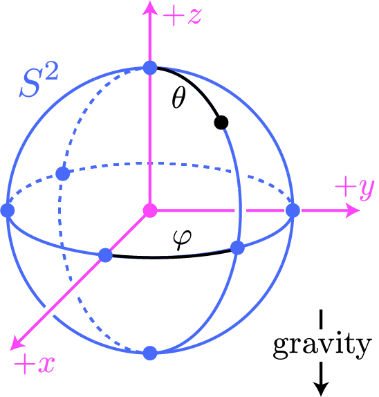
Suppose that we (locally) parametrize the sphere using the standard spherical coordinates

The angles $\varphi$ and $\theta$ (with varying domains) serve as local coordinates at every point on $S^2$, except the north and south poles. The configuration space for the system is the sphere itself $Q=S^2$, which means that the phase space is the $4$-dimensional cotangent bundle $T^\ast S^2$. The hamiltonian function $H$, which is equal to the total energy of the particle, is a smooth function defined on phase space:

\begin{equation}\notag H: T^\ast S^2 \to \bbr. \end{equation}

The first challenge that we face is in finding a formula for $H$.

Though we know that $H$ will ultimately be the total energy, it is usually quite tricky to write down the hamiltonian directly, since $H$ involves the generalized momenta $p_\varphi$ and $p_\theta$ which are often related to the usual linear momenta in a highly nontrivial way. Instead, one typically first takes a detour through Lagrange’s formulation of mechanics, writing down the lagrangian function $L$ in the form \eqref{lagrange-eqn}, and then performing a Legendre transformation \eqref{legendre-trans-eqn} to obtain $H$.

At least in situations where the system consists of particles moving about in an ambient cartesian space, the reason that it is often easier to obtain $L$ first rather than $H$ is because we can easily write down equations for kinetic and potential energies in the ambient space, and then restrict them to the tangent bundle of the configuration space. In our situation, we have the embedding of tangent bundles

\begin{equation}\label{tan-emb-eqn} T S^2 \subset T \bbr^3 \end{equation}

induced by the embedding $S^2 \subset \bbr^3$. So, our particle is constrained to move on $S^2$, but $S^2$ sits inside $\bbr^3$, and we may therefore view its trajectory as a smooth curve in $\bbr^3$. If, for simplicity, we suppose that the acceleration due to gravity is $1$, then we may take $V(z) = z$ as the scalar gravitational potential. Then, viewed as a particle moving in $\bbr^3$, the lagrangian on the tangent bundle $T \bbr^3$ is

This lagrangian will restrict to our desired lagrangian on $T S^2$ under the embedding \eqref{tan-emb-eqn} induced by the inclusion $S^2 \subset \bbr^3$.

In local coordinates, the inclusion map $\iota: S^2 \subset \bbr^3$ is given by \eqref{inclusion-eqn}. The induced inclusion \eqref{tan-emb-eqn} of tangent bundles is then realized as the pushforward

\begin{equation}\notag \iota_\ast : T S^2 \to T \bbr^3. \end{equation}

In local coordinates $(\varphi,\theta,v_\varphi,v_\theta)$ on $T S^2$ and $(x,y,z,v_x,v_y,v_z)$ on $T\bbr^3$, the pushforward $\iota_\ast$ is given by

\begin{align}\notag x &= \cos{\varphi}\sin{\theta}, &v_x &= -v_\varphi \sin{\varphi} \sin{\theta} + v_\theta \cos{\varphi}\cos{\theta}, \\y &= \sin{\varphi}\sin{\theta}, &v_y &= v_\varphi \cos{\varphi} \sin{\theta} + v_\theta \sin{\varphi} \cos{\theta}, \notag \\ z &= \cos{\theta}, &v_z &= -v_\theta \sin{\theta}. \notag \end{align}

If we substitute these expressions into \eqref{lagrange-res-eqn}, we obtain our desired lagrangian:

According to the formula \eqref{legendre-trans-eqn} for the Legendre transformation, the corresponding hamiltonian is given by

\begin{equation}\label{almost-ham-eqn} H(\varphi,\theta,p_\varphi,p_\theta) = p_\varphi v_\varphi + p_\theta v_\theta - L(\varphi,\theta,v_\varphi,v_\theta). \end{equation}

To eliminate $v_\varphi$ and $v_\theta$ in favor of $p_\varphi$ and $p_\theta$, we use that the pairs $(v_\varphi,p_\varphi)$ and $(v_\theta,p_\theta)$ are canonically conjugate, and solve the equations \eqref{conjugate-eqn} for the generalized velocities to get

\begin{equation}\notag v_\varphi = p_\varphi \csc^2{\theta} \quad \text{and} \quad v_\theta = p_\theta. \end{equation}

Then, from \eqref{lag-almost-eqn} and \eqref{almost-ham-eqn} we get our hamiltonian:

As you may then easily compute yourself, Hamilton’s equations of motion are:

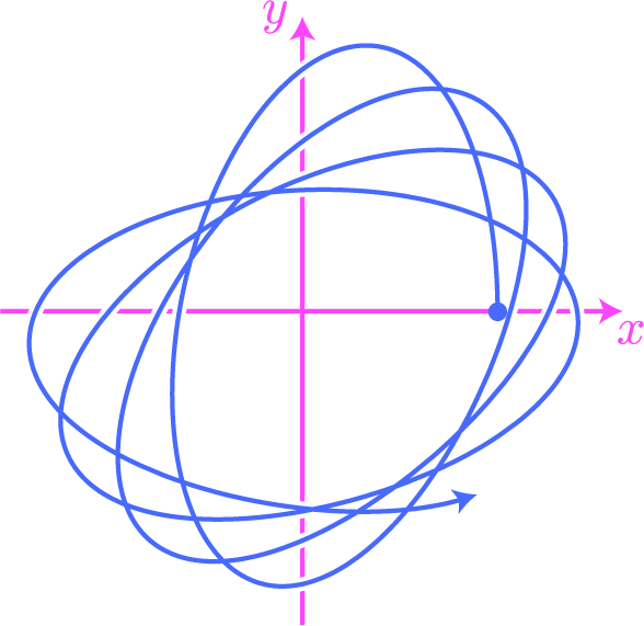
I had a computer (numerically) solve these equations with initial conditions

\begin{equation}\notag \varphi(0) = 0, \quad \theta(0) = \pi/4, \quad p_\varphi(0) = 1, \quad p_\theta(0) = 0. \end{equation}

The resulting particle trajectory, projected onto the $xy$-plane in $\bbr^3$, looks like:

The movement in the $z$-direction, plotted along the time axis, is shown in:

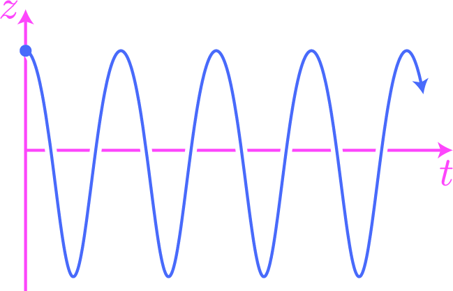
According to the initial conditions, the particle begins its trajectory on the upper hemisphere of $S^2$, sitting directly above the positive $x$-axis; this initial position is represented by the blue dots in the figures. The particle begins with no generalized momentum $p_\theta$ conjugate to the angular coordinate $\theta$, but it does have an initial positive value for the angular(!) momentum $p_\varphi$ conjugate to $\varphi$. Thus, the particle begins its trajectory by initially falling toward the bottom of the sphere while rounding the $z$-axis in the positive direction. Notice that since $\dot{p}_\varphi = 0$, the angular momentum $p_\varphi$ is conserved throughout the entire trajectory.

We now return to the general theory.

As we saw in the first section, given a mechanical system, the natural domain for Hamilton’s equations of motion is the phase space of the system, which is, by definition, the cotangent bundle $T^\ast Q$ over the configuration space $Q$ of the system. We saw that the allowable trajectories of the system, i.e., those which are solutions to Hamilton’s equations, are the integral curves of the so-called symplectic gradient of the hamiltonian function. The goal in this section is to identify the essential structures of the cotangent bundle $T^\ast Q$ that support this formalism, and to distill this structure into a new class of abstract geometric objects called symplectic manifolds.

The impulse to generalize a specific mathematical structure to a larger class of objects is often motivated by several factors, and this process of generalization and abstraction is surely one of the hallmarks of modern mathematics. When done properly, this process has both a clarifying and unifying effect. Indeed, by forcing us to identify only the essential features or structures of a given class of objects, and to strip away everything else, we may be led to a deeper and clearer understanding of those objects under study. These essential structures might then be found in another class of objects, and thus both classes may be united under a single abstract theory. Specific examples immediately spring to mind: For one, take point-set topology, which unifies geometric objects (e.g., manifolds) and analytic objects (e.g., function spaces) under one general theory.

If a mathematical abstraction does not lead to a useful or interesting theory, however, then the abstraction is of little use (whatever “useful” and “interesting” might mean). In this respect at least, mathematical theories are in analogy with physical theories, in that they both must pass a test in order to be accepted into the mainstream. Of course, for physical theories, their ultimate worth is judged by consistency with observation and predictive power.

So, in this section, we will generalize hamiltonian mechanics from cotangent bundles to live over general symplectic manifolds. This symplectic theory is extremely rich and active, and though they have their origins in physico-mechanical theories, such symplectic manifolds have become objects of study in pure mathematics. The value in these mathematical abstractions for mechanical problems might not be so apparent in this initial post, but we will see later examples of mechanical systems leading to reduced phase spaces that are not cotangent bundles; however, they do carry symplectic structures under certain conditions, and so both types of phase spaces may be united under one general symplectic theory.

Beginning the theory, we take the position that the symplectic gradient is the essential structure on a cotangent bundle $T^\ast Q$ that supports Hamilton’s mechanics. As we saw in the first section, this symplectic gradient was produced using the symplectic $2$-form

\begin{equation}\label{can2-eqn} \omega = \d q^i \wedge \d p_i \end{equation}

on $T^\ast Q$, where the $q^i$s are local coordinates on the base manifold $Q$ and the $p_i$s are the complementary “vertical” coordinates on the cotangent bundle. In other words, every covector $p\in T_q^\ast Q$ may be written as

\begin{equation}\notag p = p_i \ \d q^i. \end{equation}

That the $2$-form $\omega$ allows us to produce the (unique!) symplectic gradient $X_H$ of a hamiltonian function $H$ is a consequence of its non-degeneracy. And, though it may not be clear at this initial stage, a second crucial property of $\omega$ besides its non-degeneracy is the fact that it is closed:

\begin{equation}\notag \d \omega = 0. \end{equation}

We take these two features of the symplectic $2$-form and use them to define the main objects of study in this section:

Then, the generalization of Hamilton’s mechanics is given in:

Note that the hamiltonian function of a particular hamiltonian system is an observable of the system. The names hamiltonian function and energy function are often shortened to just hamiltonian and energy.

Of course, the first class of examples of hamiltonian systems are those which motivate the entire abstract theory: If $Q$ is the configuration space of a mechanical system and $H\in C^\infty(T^\ast Q)$ is its hamiltonian, then the triple $(T^\ast Q,\omega,H)$ is a hamiltonian system, where $\omega$ is the symplectic $2$-form defined by \eqref{can2-eqn}.

In fact, it will be worth exploring the symplectic structures on cotangent bundles $T^\ast Q$ just a little more, and to show how the symplectic form \eqref{can2-eqn} may be obtained in a coordinate-free manner. First, suppose that a point $(q,\alpha) \in T^\ast Q$ is given, where $q$ is a point of $Q$ and $\alpha \in T^\ast_q Q$ is a covector. Let

\begin{equation}\notag \pi: T^\ast Q \to Q \end{equation}

be the natural projection, and consider its pushforward

\begin{equation}\notag \pi_{\ast,(q,\alpha)} : T_{(q,\alpha)}T^\ast Q \to T_q Q. \end{equation}

Composing with $\alpha$, we get a map

\begin{equation}\notag \vartheta_{(q,\alpha)} \defeq \alpha \circ \pi_{\ast,(q,\alpha)} : T_{(q,\alpha)}T^\ast Q\to \bbr. \end{equation}

As $(q,\alpha)$ varies over all points of $T^\ast Q$, these latter maps assemble together to yield a smooth $1$-form $\vartheta$ on $T^\ast Q$ called the tautological $1$-form. We then define the standard symplectic form on $T^\ast Q$ to be

As you may easily check, $\omega$ may be given in local coordinates by the formula \eqref{can2-eqn}.

In addition to cotangent bundles, even-dimensional cartesian spaces $\bbr^{2n}$ also have symplectic structures. In fact, the space $\bbr^{2n}$ is the cotangent bundle $T^\ast \bbr^n$, at least up to diffeomorphism. If

\begin{equation}\notag (q,p) = (q^1,\ldots,q^n,p_1,\ldots,p_n) \end{equation}

are the standard (global) cartesian coordinates on $\bbr^{2n}$, then its standard symplectic form may be defined by the (global) formula \eqref{can2-eqn}.

The following fundamental theorem has the immediate corollary that even-dimensional cartesian spaces serve as the local model spaces of symplectic topology.

The special local coordinate systems \eqref{can-eqn} guaranteed by Darboux’s Theorem are called canonical local coordinates, and the form of the local expression \eqref{can3-eqn} is called the canonical form of $\omega$.

Darboux’s Theorem shows that every $2n$-dimensional symplectic manifold may be produced by gluing copies of $\bbr^{2n}$ together along open sets via sympletomorphisms. So, every symplectic manifold has a symplectic atlas, which is a smooth atlas whose transition functions are symplectomorphisms. Any object that we define on $\bbr^{2n}$ that is invariant under symplectomorphisms may therefore be transferred to live on a general symplectic manifold. It is in this sense that even-dimensional cartesian spaces serve as the local model spaces of symplectic topology, as I mentioned before the theorem.

The part of Darboux’s Theorem that claims $S$ is even-dimensional may be established by tools from elementary linear algebra; in fact, the proof of this basic result uses a technique that is called by some authors a symplectic version of the familiar Gram-Schmidt procedure, and only relies upon the fact that $\omega$ is both antisymmetric and non-degenerate (for details, see the section on Further Reading). For a fixed point $x_0\in S$, one may use this procedure to produce a basis of $T_{x_0} S$ that contains an even number of vectors and for which

\begin{equation}\label{yuppers1-eqn} \omega|_{x_0} = \alpha^i \wedge \beta_i, \end{equation}

where the $\alpha^i$s and $\beta_i$s are covectors in $T_{x_0}^\ast S$ dual to the produced basis. We may then choose an open parametrizable neighborhood $U$ centered at $x_0$ for which the associated local coordinates $(q^i,p_i)$ satisfy

\begin{equation}\label{yuppers2-eqn} \alpha^i = \d q^i|_{x_0} \quad \text{and} \quad \beta_i = \d p_i|_{x_0}. \end{equation}

We now have two closed, non-degenerate $2$-forms defined on $U$: The first is the (restriction of the) initial symplectic form $\omega$, which we will now denote by $\omega_0$, and then also the $2$-form

\begin{equation}\notag \omega_1 \defeq \d q^i \wedge \d p_i. \end{equation}

In view of \eqref{yuppers1-eqn} and \eqref{yuppers2-eqn}, the two $2$-forms $\omega_0$ and $\omega_1$ agree at $x_0$, but they may not coincide at other points $x\in U$. Therefore, something more than naive linear algebra is needed in order to establish the theorem.

The key observation is that, while the $2$-forms $\omega_0$ and $\omega_1$ are not equal at all points of $U$, they do deform into each other, perhaps on a smaller open neighborhood of $x_0$. The notion of “deformation” needed here is something called an isotopy, which is a smooth one-parameter family of self-diffeomorphisms of $S$. The desired isotopy deforming $\omega_1$ into $\omega_0$ is obtained by integrating a special time-dependent vector field to its time-dependent flow using a clever argument called Moser’s Trick. I will refer you to the section on Further Reading for references to the literature, where you may learn more about this trick.

In addition to Darboux’s Theorem, we have the following fundamental result:

We close this section with a class of examples of symplectic manifolds which—at least at first glance—have nothing to do with the phase spaces of mechanical systems: If $S$ is an embedded, oriented surface in $\bbr^3$ equipped with a “unit normal bundle” $\nu: S \to S^2$ with the property that

\begin{equation}\notag \ang{ \nu(x), v} = 0, \quad \forall x\in S, \ v\in T_xS, \end{equation}

then $S$ is a symplectic manifold. Indeed, the symplectic form on $S$ is the usual area form, given as

\begin{equation}\notag \omega_x(u,v) = \ang{ \nu(x), u \times v}, \end{equation}

where $u \times v$ denotes the cross product of the tangent vectors $u,v\in T_x S$. In particular, the sphere $S^2$ is a symplectic manifold. But $S^2$ is compact, and thus cannot be the phase space of any mechanical system.

We have defined a hamiltonian system to be a triple $(S,\omega,H)$, where $(S,\omega)$ is a symplectic manifold and the function $H\in C^\infty(S)$ is the hamiltonian. In order to produce Hamilton’s equations of motion for this system and obtain its time evolution, we require the following:

Recall that the symbol “$\iprod$” denotes the interior product of a vector field and differential form; see here for a reminder.

If $(q,p) = (q^1,\ldots,q^n,p_1,\ldots,p_n)$ are canonical local coordinates on a symplectic manifold $S$, then we have the local expression

for the symplectic gradient of a smooth function $f$. If we take $f$ to be the energy function $H$ of a hamiltonian system on $S$, then the components of $X_H$ are the partial derivatives that appear in Hamilton’s equations of motion. The remaining parts of Hamilton’s equations are obtained through the notion of an integral curve of a vector field:

We define the trajectories of a hamiltonian system to be certain integral curves:

Notice that there are several abuses of notation being committed in this definition. First, in writing \eqref{abuse}, what I really mean is that

\begin{equation}\notag (q,p) = (q^1,\ldots,q^n,p_1,\ldots,p_n) \end{equation}

are canonical local coordinates on $S$, and the right-hand side of \eqref{abuse} is short for

\begin{equation}\label{bad-eqn} \gamma(t) = \left( (q^1\circ \gamma)(t), \ldots,(q^n\circ \gamma)(t), (p_1\circ \gamma)(t),\ldots,(p_n\circ \gamma)(t) \right). \end{equation}

And second, in writing Hamilton’s equations \eqref{final-ham2-eqn}, I have omitted all evaluations at $t$, and each $(q,p)$ that appears should really be interpreted as the right-hand side of \eqref{bad-eqn}.

Symplectic gradients and Hamilton’s equations encode the laws of motion of a system which must be solved in order to discover its time evolution. It would be convenient, however, to have a geometric structure on phase space which in some sense represents the “solved” equations of motion, and encodes the time evolution directly. Such a structure is an example of the following type of general object, which makes sense on any manifold, not only the phase spaces of hamiltonian systems.

There is a tight connection between vector fields on a manifold $M$ and global flows. In particular, if $M$ happens to be the phase space of a hamiltonian system, then the flow induced by the symplectic gradient of the hamiltonian is essentially the collection of all allowable time trajectories of the system.

Before explaining this connection between vector fields and global flows, let’s examine more closely the axioms defining a global flow $\theta_t$. Though $M$ may not be related to any mechanical system, it is helpful to think of $M$ as a phase space, so that points of $M$ represent states of a system. To clarify the role of the group law

\begin{equation}\label{group2-eqn} \theta_s \circ \theta_t = \theta_{s+t}, \end{equation}

is will be helpful to define

\begin{equation}\label{art-eqn} \theta_{t_1,t_0}(x) = \theta_{t_1-t_0}(x), \quad t_0,t_1\in \bbr, \ x\in M. \end{equation}

For fixed $x_0 \in M$ and $t_0\in \bbr$, we then imagine that the point $\theta_{t_1,t_0}(x_0) \in M$ represents the state of the system beginning in the initial state $x_0$ at the initial time $t_0$, and advancing time from $t_0$ to $t_1$. Notice that

\begin{equation}\notag \theta_{t_0,t_0}(x_0) = x_0, \end{equation}

which makes sense, since the system should not change states if time is not advanced. Now, one of the corollaries of the group law \eqref{group2-eqn} is that our system is deterministic, which means that its time evolution only depends on the initial state $x_0$ at the initial time $t_0$. To explain, suppose that we advance the system to some later time $t_1 >t_0$ to obtain the state

\begin{equation}\notag x_1 = \theta_{t_1,t_0}(x_0). \end{equation}

We might imagine advancing the system once more to a time $t_2>t_1$ to obtain the state

\begin{equation}\notag x_2 = \theta_{t_2,t_1}(x_1). \end{equation}

Then, determinism in this context means that the state $x_2$ does not depend on the intermediate state $x_1$ and intermediate time $t_1$, and could be obtained directly from the initial state and time:

\begin{equation}\notag x_2 = \theta_{t_2,t_1}(x_1) = \left( \theta_{t_2,t_1} \circ \theta_{t_1,t_0}\right)(x_0)= \theta_{t_2- t_0}(x_0) = \theta_{t_2,t_0}(x_0). \end{equation}

Note that the definition \eqref{art-eqn} says that the time evolution from $t_0$ to $t_1$ does not depend on the specific values of $t_0$ and $t_1$, but rather only on the difference $t_1-t_0$; this is a form of time independence of the global flow $\theta_t$. The group law was the crucial ingredient needed to show that the definition \eqref{art-eqn} led to a deterministic time evolution, and thus the group law can be understood as a form of time independence. It is worth contrasting our discussion here with the case of time-dependenent flows; some references for these latter gadgets are given in the section on Further Reading.

So, our discussion here shows that the curves

\begin{equation}\label{flow-curve-eqn} t \mapsto \theta_t(x) \end{equation}

obtained from a global flow $\theta_t$ on a manifold $M$ are interesting objects. These smooth curves provide the mechanism to move from a global flow to a vector field:

The infinitesimal generator $X$ is smooth. You might try to prove this on your own; otherwise, see the references in the section on Further Reading.

Given a flow $\theta_t$ and its infinitesimal generator $X$, one recovers the curves \eqref{flow-curve-eqn} from $X$ by taking integral curves. Formally:

The desired equation is an easy consequence of the group law and the chain rule. Indeed, beginning with the definition of the infinitesimal flow, we compute

\begin{equation}\notag X(\theta_t(x)) = \frac{\d}{\d s} \Big|_{s=0} \theta_s(\theta_t(x)) = \frac{\d}{\d s}\Big|_{s=0} \theta_{t+s}(x) = \frac{\d}{\d s} \Big|_{s=t} \theta_s(x), \end{equation}

which is what we wanted to prove. Q.E.D.

So, through its infinitesimal generator, one may obtain a vector field from any global flow. What about the other direction—can one generate a global flow from any vector field? We will begin to answer this question by first defining special types of integral curves:

Now, let $M$ be a smooth manifold. A flow domain is an open subset $D$ of $\bbr \times M$ with the property that, for each $x\in \bbr$, the $1$-dimensional “slice”

\begin{equation}\notag (\bbr \times \{x\}) \cap D, \end{equation}

is an open interval containing $0$. Then, a local flow on $M$ is a smooth map

\begin{equation}\notag \theta: D \to M, \quad (t,x) \mapsto \theta_t(x), \end{equation}

defined on some flow domain $D$, such that $\theta_0(x)=x$ for all $(0,x)\in D$ and

\begin{equation}\notag (\theta_s \circ \theta_t)(x) = \theta_{s+t}(x) \end{equation}

for all $(t,x)\in D$ and $s\in \bbr$ for which $(s,\theta_t(x)),(s+t,x)\in D$. The local flow $\theta$ is said to be maximal if it cannot be extended to a local flow defined on a larger flow domain $D’$ containing $D$.

An infinitesimal generator $X$ of a local flow $\theta$ is defined just as it is for global flows, and the integral curves of $X$ are exactly the curves $t\mapsto \theta_t(x)$, for fixed $x$.

For a proof, see the references listed in the section on Further Reading.

One might inquire about conditions on the underlying manifold that guarantee completeness of all vector fields. Such a condition is identified in:

Again, for a proof, see the section on Further Reading.

Let $X$ be a vector field on a manifold $M$ and suppose for simplicity that it is complete and generates a global flow $\theta_t$. If $M$ happens to be the phase space of a mechanical system and $\theta_t$ encodes the time evolution of the system, then one of the goals in our study is to identify conserved quantities, i.e., quantities that do not change or vary along the curves

\begin{equation}\label{curve-eqn} t\mapsto \theta_t(x), \end{equation}

for fixed $x\in M$. In the most general case, by “quantity” we might mean a tensor field on $M$ of arbitrary type; however, for our purposes it will suffice to narrow our focus to tensors of particular types, namely functions, differential forms, and vector fields.

There is an obvious notion of what it should mean for a function $f\in C^\infty(M)$ to be conserved along the curve \eqref{curve-eqn}; indeed, this will be the case when $f$ is constant along the curve,

\begin{equation}\label{constant-eqn} f(x) = f(\theta_t(x)) \end{equation}

for all $t\in \bbr$. If we require this identity to hold for all $x\in M$, then it may be rewritten concisely as

\begin{equation}\label{constant2-eqn} f = \theta^\ast_t f, \quad \forall t\in \bbr, \end{equation}

where $\theta_t^\ast$ is the pullback map of the self-diffeomorphism $\theta_t: M \to M$. But what should it mean for a differential form $\omega$ to be conserved? Clearly, it does not make sense to mimic \eqref{constant-eqn} and write

\begin{equation}\notag \omega_x = \omega_{\theta_t(x)}, \end{equation}

since the left- and right-hand sides live in different vector spaces. Rather, the key is to use \eqref{constant2-eqn} as inspiration, and declare that $\omega$ is conserved under the flow $\theta_t$ provided that

\begin{equation}\label{constant3-eqn} \omega = \theta^\ast_t \omega, \quad \forall t\in \bbr. \end{equation}

If $Y$ is a second vector field on $M$, then by mimicking \eqref{constant2-eqn} and \eqref{constant3-eqn}, we should say that $Y$ is conserved under the flow $\theta_t$ provided that

\begin{equation}\label{constant4-eqn} Y = \theta^\ast_t Y, \quad \forall t\in \bbr. \end{equation}

However, in contrast to the pullbacks in \eqref{constant2-eqn} and \eqref{constant3-eqn}, which are often encountered early in one’s study of smooth manifolds, the pullback of a vector field is less ubiquitous and therefore deserves a careful definition:

In view of the definition in this exercise, the right-hand side of \eqref{constant4-eqn} is defined by the equalities

\begin{equation}\notag (\theta^\ast_t Y)_x = (\theta_{-t})_{\ast,\theta_t(x)} \left( Y_{\theta_t(x)} \right), \quad t\in \bbr, \ x\in M. \end{equation}

Let’s collect all three of our definitions together and place them into a single box for convenient reference:

Nothing in this section really requires the vector field $X$ to be complete, but then one must use caution in writing equalities like $f = \theta_t^\ast f$, taking care to precisely identify the domain of the local flow. To avoid these minor annoyances, I will continue to assume that $X$ is complete, and leave it up to you to translate all the results to local flows.

One of the main lessons of differential calculus is that a conserved (or constant) quantity is often identified by the vanishing of a derivative of some sort. My main goal in this section is to cook up a type of derivative with respect to $X$, denoted $\call_X$, that applies to the three types of quantities we are studying:

\begin{equation}\label{three-eqn} \call_X f, \quad \call_X \omega, \quad \call_X Y, \end{equation}

These derivatives are all called Lie derivatives, though one might also call them flow derivatives, since each of their definitions utilizes the flow $\theta_t$ generated by $X$. Each derivative is an object of the same type, so that, for example, $\call_X f$ is a smooth function on $M$. The key property of these derivatives will be that their vanishing signals a conserved quantity.

The definitions, all in one shot, are:

Though the definitions are nice and concise, make sure that you understand exactly what they mean. For example, if we were being more precise, we would define the Lie derivative $\call_X f$ pointwise by setting

\begin{equation}\notag (\call_Xf)(x) = \lim_{\dev \to 0} \frac{(\theta_\dev^\ast f)(x) - f(x)}{\dev}, \end{equation}

for $x\in M$.

There is obvious redundancy in the definition, essentially repeating the same definition three times. This redundancy could be eliminated by first defining the pullback of a tensor field of arbitrary type (along a diffeomorphism), and then defining the Lie derivative of such a tensor field in the manner above.

The next exercise shows that the Lie derivative $\call_X f$ is a familiar object.

Though Lie derivatives are defined as derivatives at time $t=0$, they may be used to compute derivatives at other times as well. This is the content of the following important result.

The main ingredient in the proofs is a trick that changes the derivative evaluated at $s=t$ to the derivative evaluated at $s=0$, which we already saw in the previous section. Here’s how it goes, starting with the right-hand side of the first desired equality:

\begin{equation}\label{cute-eqn} \frac{\d}{\d s}\Big|_{s=t} \theta^\ast_s f = \frac{\d}{\d s}\Big|_{s=0} \theta^\ast_{s+t} f = \frac{\d}{\d s}\Big|_{s=0} \theta^\ast_{t} \theta^\ast_s f = \theta^\ast_t \call_Xf. \end{equation}

Essentially the same argument works for the other two desired equalities. I suggest that you work through them in detail, to see how all the ingredients are used. After that, we may declare: Q.E.D.

The following corollary is the main result of this section, which we will use quite often.

Computing Lie derivatives of differential forms is often made easier by leveraging the following formula; for a proof, see the section on Further Reading.

In this short section, we finish the post by proving a pair of fundamental results in the hamiltonian formalism:

1. The flows of hamiltonian vector fields consist of symplectomorphisms.
2. The Conservation of Energy Theorem.

Both of these results deal with conserved quantities (a $2$-form in the first case, a function in the second), and so we will be able to use the Lie derivatives defined and studied in the previous section.

First, we define three special types of vector fields on symplectic manifolds.

The definition of a symplectic vector field might initially be quite opaque; the next theorem hopefully clarifies the situation. This theorem also explains how the three types of vector fields just defined are related to each other.

For the first statement, recall that $\omega$ is conserved along the flow of $X$ if and only if $\call_X \omega=0$. But, by Cartan’s Magic Formula and the closedness of $\omega$, we have

\begin{equation}\notag \call_X \omega = \d (X\iprod \omega). \end{equation}

The desired result then follows. Now:

As an immediate corollary to the theorem, we get the first fundamental result mentioned at the beginning of this section:

Indeed, since the vector field $X_f$ is symplectic, the symplectic form $\omega$ is conserved along the flow $\theta_t$. But this means that $\omega = \theta_t^\ast \omega$, which is the definition of a symplectomorphism. Q.E.D.

We end this post with the second of the fundamental results mentioned above. The powerful tools and techniques we have built up to this point render the proof extremely short.

We need to prove that the Lie derivative $\call_{X_H} H$ vanishes. But this follows from the following simple computation:

\begin{equation}\notag \call_{X_H}H = \d H \left( X_H \right) = (X_H \iprod \omega)(X_H) = \omega(X_H,X_H) = 0. \end{equation}

The first equality is the definition of the Lie derivative of a smooth function, the second uses the definition of $X_H$, the third uses the definition of the interior product, while the fourth follows from antisymmetry of $\omega$. Q.E.D.

The standard reference for a mathematical treatment of hamiltonian mechanics is Abraham and Marsden’s textbook.¹ The symplectic theory is treated in detail there.

A good reference for symplectic manifolds in mathematics is McDuff and Salamon’s text², which contains a huge amount of material. Two shorter (but still book-length) introductions are given in Berndt’s book,³ and also Cannas da Silva’s,⁴ while a much shorter introduction is the last chapter of Lee’s book⁵ on smooth manifolds. All of these texts contain detailed proofs of the fundamental Darboux Theorem and “Moser’s Trick.”

Lee’s book contains a thorough treatment of vector fields and flows (both time-independent and dependent), including a proof of the Fundamental Theorem on Flows.

A proof of Cartan’s Magic Formula may also be found in Lee’s book.